Chapter 10 Multivariate Regression and Hypothesis Testing

10.1 Basic Multivariate Regression

Basic syntax: `

myReg <- lm(formula, data)

where formula describes the model to be fit and data is the data frame containing the data to be used in fitting the model. Example,

myReg <- lm(y ~ X1 + X2, data = women)

Here, the formula is y ~ X1 + X2 There are some symbols that allow to modify the formula conveniently.

Symbols in Regression Analysis:

Symbol	Usage	Example
`~`	Separates dep. and indep. variables	`y ~ X1 + X2`
`~`	Separates dep. and indep. variables	`y ~ X1 + X2`
`:`	Provides interaction terms	`y ~ X1 + X2 + X1:X2`
`*`	All interaction terms	`y ~ X1X2X3`
`^`	All interaction terms up to a degree	`y ~ (X1 + X2 + X3)^2`
`.`	Placeholder for all other variables	`y ~ .`
`-`	Removes a term from the equation	`y ~ (X1 + X2)^2 - X1:X2`
`-1`	Suppresses the intercept term	`y ~ X1 - 1`
`I()`	`()` are interpreted arithmetically	`y ~ X1 + I((X1+X2)^2)`

Note that

y ~ X1 + (X2+X3)^2
## y ~ X1 + (X2 + X3)^2

would produce

y ~ X1 + X2 + X3 + X2:X3
## y ~ X1 + X2 + X3 + X2:X3

On the other hand,

y ~ X1 + I((X2+X3)^2)
## y ~ X1 + I((X2 + X3)^2)

will produce a regression with two independent variables: \(X1\) and \((X2+X3)^2\).

Once an object containing the regression output is created with lm() we can extract various information using the following functions:

Functions
`summary()`	`anova()`
`coefficients()`	`vcov()`
`confid()`	`AIC()`
`fitted()`	`plot()`
`residuals()`	`predict()`

All these functions can be used with lm().

10.2 An Extended Example

For this example, we will use the state.x77 dataset in the base package, which provides murder rates and other characteristics of the states, including population, illiteracy rate, average income, and frost levels (mean number of days below freezing).

Let’s save the data as a data frame first:

states <- as.data.frame(state.x77[,c("Murder", "Population",
                                     "Illiteracy", "Income", "Frost")])

A simple(bivariate) regression with the plot

myReg <- lm(Murder ~ Illiteracy, data=states)

plot(states$Illiteracy,states$Murder,
xlab="Illiteracy",
ylab="Murder")

abline(myReg)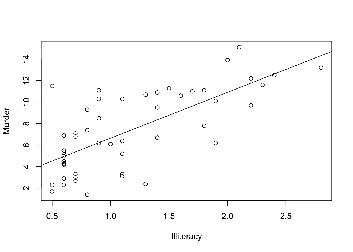

Include a polynomial term

myReg <- lm(Murder ~ Illiteracy + I(Illiteracy^2), data=states)

plot(states$Illiteracy,states$Murder,
xlab="Illiteracy",
ylab="Murder")

lines(states$Illiteracy,fitted(myReg))

Note that here we have used another method to include the fitted regression line because abline() works only in a single variable case.

A multiple linear regression

myReg <- lm(Murder ~ Population + Illiteracy + Income + Frost, data=states)

Since we are using all the variables in the data frame states, we could alternatively run this regression simply as

myReg1 <- lm(Murder ~ ., data=states)

A multiple linear regression with an interaction term

myReg <- lm(Murder ~ Population + Illiteracy + Income + Frost 
                                  + Population:Illiteracy, data=states)

Recall that a significant interaction between two predictor variables tells you that the relationship between one predictor and the response variable depends on the level of the other predictor.

In order to evaluate the statistical assumptions behind the OLS method a standard approach is to apply plot() function to the object created by lm():

myReg <- lm(Murder ~ Population + Illiteracy + Income + Frost, data=states)
par(mfrow = c(2,2))
plot(myReg)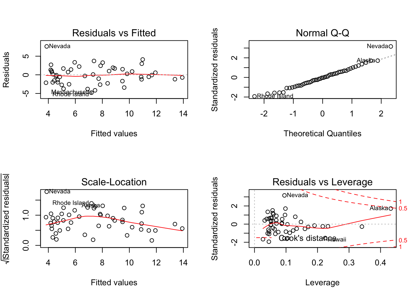

where par(mfrow=c(2,2)) statement is used to combine the four plots produced by the plot() function into a \(2\times 2\) graph.

Interpretation of four plots:

Upper left plot provides information about the model specification, in this case whether the linear model is an appropriate specification.

Upper right plot provides information about the normality assumption

Lower left plot provides information about the homoscedasticity assumption

Lower right plot provides information about the individual observations to help identifying outliers, leverage values and influential observations

Instead of going into details of these four plots, we will use Car package as a better alternative for checking regression diagnostics.

10.3 Regression Diagnostics with `Car` package

Functions for Regression Diagnostics in Car package

Function	Usage
`qqPlot()`	Quantile comparisons plot
`durbinWatsonTest()`	DW test for autocorrelation
`crPlots()`	Component plus residual plots
`ncvTest()`	Score test for nonconstant error variance
`spreadLevelPlot()`	Spread-level plots
`outlierTest()`	Bonferroni outlier test
`avPlots()`	Added variable plots
`influencePlot()`	Regression influence plots
`scatterplot()`	Enhanced scatter plots
`scatterplotMatrix()`	Enhanced scatter plot matrices
`vif()`	Variance Inflation Factors

10.4 Normality

The qqPlot() function plots the studentized residuals against a \(t\) distribution with \(n-k-1\) degrees of freedom, where \(n\) is the sample size and \(k\) is the number of regression parameters (including the intercept). Applying this function to our states example

library(car)
states <- as.data.frame(state.x77[,c("Murder", "Population",
                                     "Illiteracy", "Income", "Frost")])
myReg <- lm(Murder ~ Population + Illiteracy + Income + Frost, data=states)

qqPlot(myReg, labels=row.names(states), id.method="identify",
       simulate=TRUE, main="Q-Q Plot")

Options:

simulate=TRUE provides a 95% confidence envelope
id.method ="identify" makes the plot interactive. Better to turn it off if there are some follow up codes.

The following residplot() function generates a histogram of the studentized residuals and superimposes a normal curve, kernel-density curve, and rug plot. It doesn’t require the car package.

residplot <- function(myReg, nbreaks=10) {
  z <- rstudent(myReg)
  hist(z, breaks=nbreaks, freq=FALSE,
       xlab="Studentized Residual",
       main="Distribution of Errors")
  rug(jitter(z), col="brown")
  curve(dnorm(x, mean=mean(z), sd=sd(z)),
        add=TRUE, col="blue", lwd=2)
  lines(density(z)$x, density(z)$y,
        col="red", lwd=2, lty=2)
  legend("topright",
         legend = c( "Normal Curve", "Kernel Density Curve"),
         lty=1:2, col=c("blue","red"), cex=.7)
}

residplot(myReg)

10.5 Autocorrelation

To apply the Durbin-Watson test to our multiple-regression problem we can use the following code:

durbinWatsonTest(myReg)
##  lag Autocorrelation D-W Statistic p-value
##    1      -0.2006929      2.317691    0.26
##  Alternative hypothesis: rho != 0

The durbinWatsonTest() function uses bootstrapping to derive p-values, therefore you’ll get a different test statistics each time you run the test unless you add the option simulate=FALSE

durbinWatsonTest(myReg, simulate=TRUE)
##  lag Autocorrelation D-W Statistic p-value
##    1      -0.2006929      2.317691   0.226
##  Alternative hypothesis: rho != 0

10.6 Linearity

By using component plus residual plots we can check whether there is any systematic departure from the linear specification.This plot is produced by the crPlots() function in the car package:

library(car)
crPlots(myReg)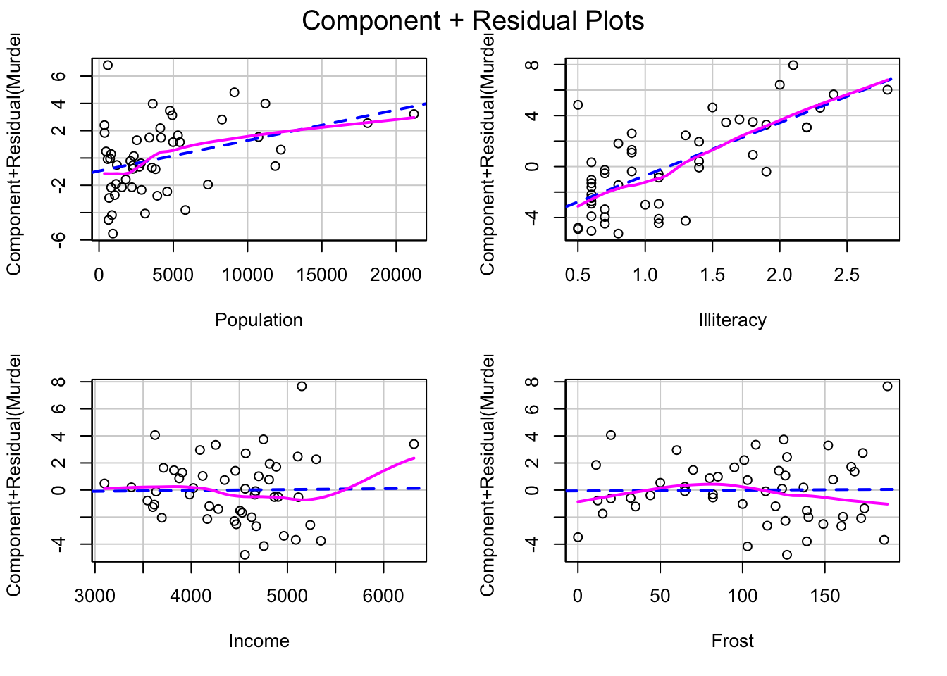

It produces one plot for each independent variable. Nonlinearity in any of these plots might suggest to add polynomial terms, transform some of the variables or use some other nonlinear specification.

10.7 Homoscedasticity

The Car function ncvTest() gives a score test to assess the homoscedasticity

library(car)
ncvTest(myReg)
## Non-constant Variance Score Test 
## Variance formula: ~ fitted.values 
## Chisquare = 1.746514, Df = 1, p = 0.18632

Here the null hypothesis is constant error variance and the alternative hypothesis is that the error variance changes with the level of the fitted values.

We can also look at the scatter plot of the absolute standardized residuals versus the fitted values and superimposes a line of best fit. This plot is produced by the spreadLevelPlot() function in Car.

library(car)
spreadLevelPlot(myReg)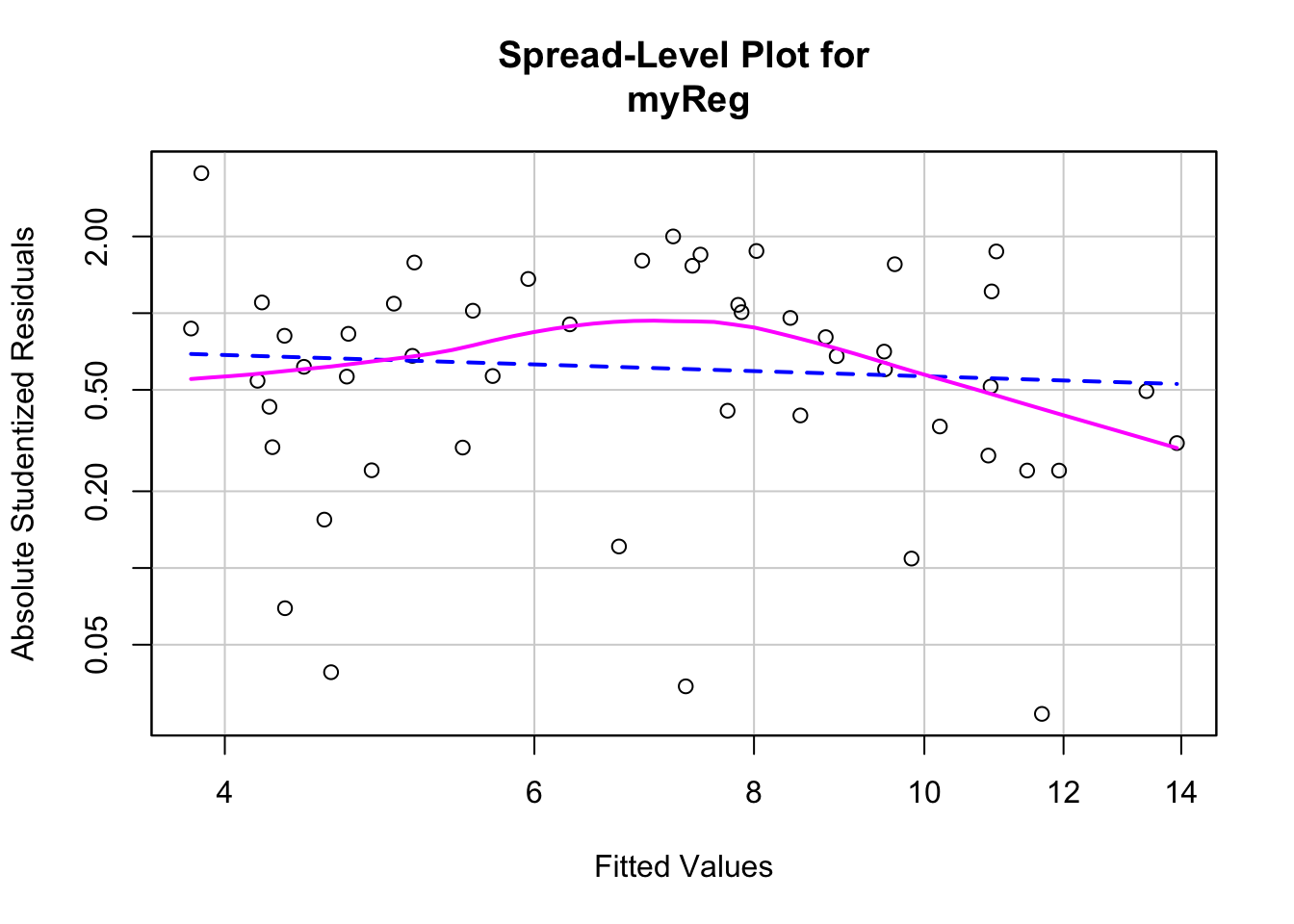

## 
## Suggested power transformation:  1.209626

This function also provides a suggested power transformation for the dependent variable. In case of homoscedasticity, the suggested transformation should be around 1.

10.8 Multicollinearity

Multicollinearity can be detected using a statistic called the variance inflation factor (VIF). For any predictor variable, the square root of the VIF indicates the degree to which the confidence interval for that variable’s regression parameter is expanded relative to a model with uncorrelated predictors. VIF values are provided by the vif() function in the car package. As a general rule, \(vif > 4\) indicates a multicollinearity problem.

library(car)
vif(myReg)
## Population Illiteracy     Income      Frost 
##   1.245282   2.165848   1.345822   2.082547

10.9 Diagnostics Summary

Now, let’s summarize all these test in the same list:

library(car)
states <- as.data.frame(state.x77[,c("Murder", "Population",
                                     "Illiteracy", "Income", "Frost")])
myReg <- lm(Murder ~ Population + Illiteracy + Income + Frost, data=states)

#Normality
qqPlot(myReg, labels=row.names(states), simulate=FALSE, main="Q-Q Plot")

#Autocorrelation
durbinWatsonTest(myReg)

#Linearity
crPlots(myReg)

#Homoscedasticity
ncvTest(myReg)
spreadLevelPlot(myReg)

#Multicollinearity
vif(myReg)

Check also gvlma() function in the gvlma package written by Pena and Slate (2006). This function performs a global validation of linear model assumptions as well as separate evaluations of skewness, kurtosis, and heteroscedasticity

#A Global Test of Model Assumptions
library(gvlma)
global <- gvlma(myReg) 
summary(global)