Chapter 9 Simple Regression
In this chapter we are basically replicate all the empirical results of Chapter 4 and 5 in Stock and Watson. First we are going to use our own functions and then we will try to take advantage of built-in R functions.
9.1 Data Preparation
Without data we can do nothing in econometrics, so let’s read in our data and prepare it for the analysis.
California test scores data are already included in a few R packages, one of which is car package. Using this package let’s read in our data:
#install.packages("AER")
library("AER")
# which data sets are included?
data()

# California data set is CASchools, let's load it
data(CASchools)

# To see the descriptions of the variables
help("CASchools", package = "AER")
Now we have the data loaded in the current session.
To make a sense of data look at the summary:
summary(CASchools)
##    district            school                  county      grades
##  Length:420         Length:420         Sonoma     : 29   KK-06: 61
##  Class :character   Class :character   Kern       : 27   KK-08:359
##  Mode  :character   Mode  :character   Los Angeles: 27
##                                        Tulare     : 24
##                                        San Diego  : 21
##                                        Santa Clara: 20
##                                        (Other)    :272
##     students          teachers          calworks          lunch
##  Min.   :   81.0   Min.   :   4.85   Min.   : 0.000   Min.   :  0.00
##  1st Qu.:  379.0   1st Qu.:  19.66   1st Qu.: 4.395   1st Qu.: 23.28
##  Median :  950.5   Median :  48.56   Median :10.520   Median : 41.75
##  Mean   : 2628.8   Mean   : 129.07   Mean   :13.246   Mean   : 44.71
##  3rd Qu.: 3008.0   3rd Qu.: 146.35   3rd Qu.:18.981   3rd Qu.: 66.86
##  Max.   :27176.0   Max.   :1429.00   Max.   :78.994   Max.   :100.00
##
##     computer       expenditure       income          english
##  Min.   :   0.0   Min.   :3926   Min.   : 5.335   Min.   : 0.000
##  1st Qu.:  46.0   1st Qu.:4906   1st Qu.:10.639   1st Qu.: 1.941
##  Median : 117.5   Median :5215   Median :13.728   Median : 8.778
##  Mean   : 303.4   Mean   :5312   Mean   :15.317   Mean   :15.768
##  3rd Qu.: 375.2   3rd Qu.:5601   3rd Qu.:17.629   3rd Qu.:22.970
##  Max.   :3324.0   Max.   :7712   Max.   :55.328   Max.   :85.540
##
##       read            math
##  Min.   :604.5   Min.   :605.4
##  1st Qu.:640.4   1st Qu.:639.4
##  Median :655.8   Median :652.5
##  Mean   :655.0   Mean   :653.3
##  3rd Qu.:668.7   3rd Qu.:665.9
##  Max.   :704.0   Max.   :709.5
##
And then the look at the first few rows:
head(CASchools)
##   district                          school  county grades students
## 1    75119              Sunol Glen Unified Alameda  KK-08      195
## 2    61499            Manzanita Elementary   Butte  KK-08      240
## 3    61549     Thermalito Union Elementary   Butte  KK-08     1550
## 4    61457 Golden Feather Union Elementary   Butte  KK-08      243
## 5    61523        Palermo Union Elementary   Butte  KK-08     1335
## 6    62042         Burrel Union Elementary  Fresno  KK-08      137
##   teachers calworks   lunch computer expenditure    income   english  read
## 1    10.90   0.5102  2.0408       67    6384.911 22.690001  0.000000 691.6
## 2    11.15  15.4167 47.9167      101    5099.381  9.824000  4.583333 660.5
## 3    82.90  55.0323 76.3226      169    5501.955  8.978000 30.000002 636.3
## 4    14.00  36.4754 77.0492       85    7101.831  8.978000  0.000000 651.9
## 5    71.50  33.1086 78.4270      171    5235.988  9.080333 13.857677 641.8
## 6     6.40  12.3188 86.9565       25    5580.147 10.415000 12.408759 605.7
##    math
## 1 690.0
## 2 661.9
## 3 650.9
## 4 643.5
## 5 639.9
## 6 605.4
Recall that we have been working with two variables so far STR (student teacher ratio) and TestScore, which is defined as the average of math and reading scores. CASchools is a data frame so we can compute the variables of interest as follows
STR <- CASchools$students / CASchools$teachers
TestScore <- (CASchools$read + CASchools$math)/2plot( TestScore ~ STR,
xlab = "Student Teacher Ratio (STR)",
ylab = "Test Score",
main = "STR vs Test Score",
pch = 20,
cex = 2,
col = "blue")
9.2 Simple Regression: theory
The population regression model, \[ Y_i = \beta_0 + \beta_1 X_i + u_i \] The sample regression line, \[ \widehat{Y}_i = \widehat{\beta}_0 + \widehat{\beta}_1 X_i \] where \[ \begin{aligned} \widehat{\beta}_1 &= \frac{\sum_{i = 1}^{n}(X_i - \overline{X})(Y_i - \overline{Y})}{\sum_{i = 1}^{n}(X_i - \overline{X})^2} = \frac{s_{xy}}{s_{x}} \\ \widehat{\beta}_0 &= \overline{Y} - \widehat{\beta}_1 \overline{X} \end{aligned} \] and OLS residuals: \[ \widehat{u}_i = Y_i - \widehat{Y}_i \] ## Simple Regression: computation First some auxiliary computations:
n <- length(STR)
x <- STR
y <- TestScore
s_xy <- (sum((x - mean(x))*(y - mean(y))))/(n - 1)
s_x <- (sum((x - mean(x))^2))/(n - 1)
s_y <- (sum((y - mean(y))^2))/(n - 1)Calculate \(\widehat{\beta}_0\) and \(\widehat{\beta}_1\):
beta_1_hat <- s_xy / s_x
beta_0_hat <- mean(y) - beta_1_hat * mean(x)
myCoefficients <- c(beta_0_hat, beta_1_hat)
myCoefficients
## [1] 698.932949 -2.279808Therefore, the sample regression line is \[ \widehat{Y} = 698.93 + (-2.28) X. \]
And everything else:
y_hat <- beta_0_hat + beta_1_hat * x # predictions
u_hat <- y - y_hat # residuals
TSS <- sum((y - mean(y))^2)
ESS <- sum((y_hat - mean(y))^2)
SSR <- TSS - ESS
R_sq <- ESS/TSS
ser <- sqrt(sum(u_hat^2)/(n-2)) # standard error of reg.
c(R_sq, ser)
## [1] 0.05124009 18.580966699.3 Simple Regression: using the lm Function
So far we have done regression by deriving the least squares estimates, then writing simple R commands to perform the necessary calculations. Since this is such a common task, this functionality that is built directly into R via the lm() function.
The lm() function is used to fit linear models which actually account for a broader class of models than simple linear regression, but we will use SLR as our first demonstration of lm(). The lm() function will be one of our most commonly used tools, so you may want to take a look at the documentation by using ?lm. You’ll notice there is a lot of information there, but we will start with just the very basics. This is documentation you will want to return to often.
We’ll continue using the cars data, and essentially use the lm() function to check the work we had previously done.
ca_model <- lm(TestScore ~ STR)This line of code fits our very first linear model. We use the TestScore ~ STR syntax to tell R we would like to model the response variable TestScore as a linear function of the predictor (independent) variable STR. In general, you should think of the syntax as response ~ predictor.
The variable ca_model now contains a wealth of information, and we will now see how to extract and use that information. The first thing we will do is simply output whatever is stored immediately in the variable ca_model.
ca_model
##
## Call:
## lm(formula = TestScore ~ STR)
##
## Coefficients:
## (Intercept) STR
## 698.93 -2.28We see that it first tells us the formula we input into R, that is lm(formula = TestScore ~ STR). We also see the coefficients of the model. We can check that these are what we had calculated previously:
c(beta_0_hat, beta_1_hat) # estimations from manual computations
## [1] 698.932949 -2.279808Next, it would be nice to add the fitted line to the scatterplot. To do so we will use the abline() function:
plot( TestScore ~ STR,
     xlab = "Student Teacher Ratio (STR)",
     ylab = "Test Score",
     main = "STR vs Test Score",
     pch  = 20,
     cex  = 2,
     col  = "blue")
abline(ca_model, lwd = 3, col = "green")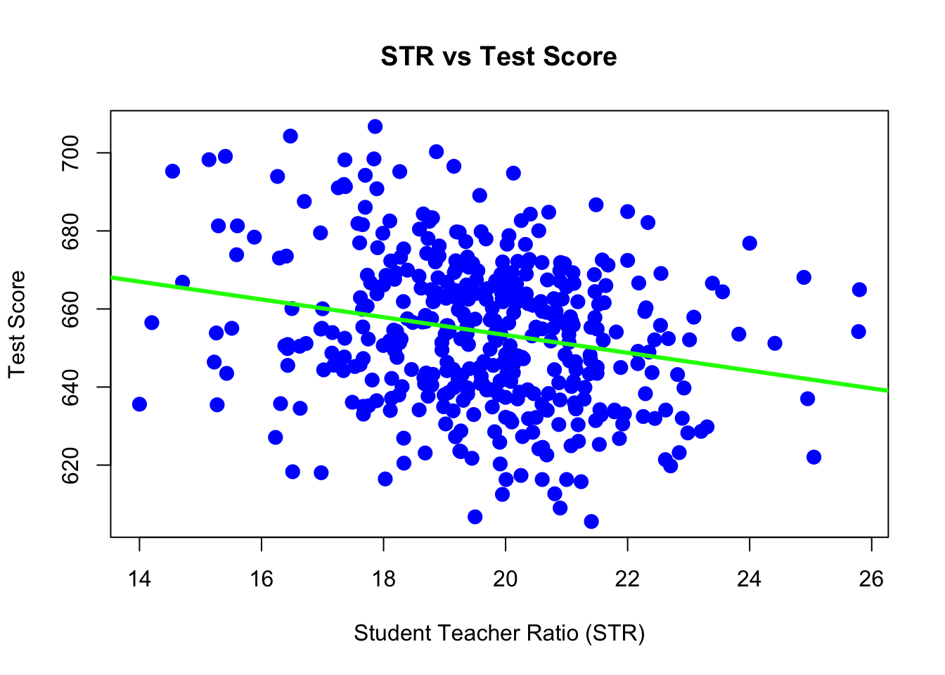 The
The abline() function is used to add lines of the form \(a + bx\) to a plot. (Hence abline.) When we give it ca_model as an argument, it automatically extracts the regression coefficient estimates (\(\widehat{\beta}_0\) and \(\widehat{\beta}_1\)) and uses them as the slope and intercept of the line. Here we also use lwd to modify the width of the line, as well as col to modify the color of the line.
The “thing” that is returned by the lm() function is actually an object of class lm which is a list. The exact details of this are unimportant unless you are seriously interested in the inner-workings of R, but know that we can determine the names of the elements of the list using the names() command:
names(ca_model)
##  [1] "coefficients"  "residuals"     "effects"       "rank"
##  [5] "fitted.values" "assign"        "qr"            "df.residual"
##  [9] "xlevels"       "call"          "terms"         "model"
We can then use this information to, for example, access the coefficients using the $ operator:
ca_model$coefficients
## (Intercept)         STR
##  698.932949   -2.279808
and residuals
ca_model$residuals[1:5]   # the first 5 residual
##         1         2         3         4         5
##  32.65260  11.33917 -12.70686 -11.66198 -15.51590
An R function that is useful in many situations is summary(). We see that when it is called on our model, it returns a good deal of information:
summary(ca_model)
##
## Call:
## lm(formula = TestScore ~ STR)
##
## Residuals:
##     Min      1Q  Median      3Q     Max
## -47.727 -14.251   0.483  12.822  48.540
##
## Coefficients:
##             Estimate Std. Error t value Pr(>|t|)
## (Intercept) 698.9329     9.4675  73.825  < 2e-16 ***
## STR          -2.2798     0.4798  -4.751 2.78e-06 ***
## ---
## Signif. codes:  0 '***' 0.001 '**' 0.01 '*' 0.05 '.' 0.1 ' ' 1
##
## Residual standard error: 18.58 on 418 degrees of freedom
## Multiple R-squared:  0.05124,    Adjusted R-squared:  0.04897
## F-statistic: 22.58 on 1 and 418 DF,  p-value: 2.783e-06
By the end of the course, you will know what every value here is used for. For now, you should immediately notice the coefficient estimates, and you may recognize the \(R^2\) value we saw earlier.
The summary() command also returns a list, and we can again use names() to learn more about the elements of this list:
names(summary(ca_model))
##  [1] "call"          "terms"         "residuals"     "coefficients"
##  [5] "aliased"       "sigma"         "df"            "r.squared"
##  [9] "adj.r.squared" "fstatistic"    "cov.unscaled"
So, for example, if we wanted to directly access the value of \(R^2\), instead of copy and pasting it out of the printed statement from summary(), we could do so by
summary(ca_model)$r.squared
## [1] 0.05124009
Another value we may want to access is \(SER\), which R calls sigma:
summary(ca_model)$sigma
## [1] 18.58097
Note that this is the same result seen earlier as se. You may also notice that this value was displayed above as a result of the summary() command, which R labeled the “Residual Standard Error.” \[
\text{SER} = \sqrt{\frac{1}{n - 2}\sum_{i = 1}^n u_i^2}
\] We can also obtain a more compact summary of the results:
summary(ca_model)$coefficients
##               Estimate Std. Error   t value      Pr(>|t|)
## (Intercept) 698.932949  9.4674911 73.824516 6.569846e-242
## STR          -2.279808  0.4798255 -4.751327  2.783308e-06
The summary of the model just for the intercept:
summary(ca_model)$coefficients[1, ]
##      Estimate    Std. Error       t value      Pr(>|t|)
##  6.989329e+02  9.467491e+00  7.382452e+01 6.569846e-242
The summary of the model just for the slope:
summary(ca_model)$coefficients[2, ]
##      Estimate    Std. Error       t value      Pr(>|t|)
## -2.279808e+00  4.798255e-01 -4.751327e+00  2.783308e-06
In summary, the following code stores the information of summary(ca_model)$coefficients in a new variable ca_model_info, then extracts each element into a new variable which describes the information it contains.
ca_model_info = summary(ca_model)$coefficients

beta_0_hat      = ca_model_info[1, 1] # Estimate
beta_0_hat_se   = ca_model_info[1, 2] # Std. Error
beta_0_hat_t    = ca_model_info[1, 3] # t value
beta_0_hat_pval = ca_model_info[1, 4] # Pr(>|t|)

beta_1_hat      = ca_model_info[2, 1] # Estimate
beta_1_hat_se   = ca_model_info[2, 2] # Std. Error
beta_1_hat_t    = ca_model_info[2, 3] # t value
beta_1_hat_pval = ca_model_info[2, 4] # Pr(>|t|)
We can then verify some equivalent expressions: the \(t\) test statistic for \(\widehat{\beta}_1\) and the two-sided p-value associated with that test statistic.
(beta_1_hat - 0) / beta_1_hat_se
## [1] -4.751327
beta_1_hat_t
## [1] -4.751327
2 * pt(abs(beta_1_hat_t), df = length(resid(ca_model)) - 2, lower.tail = FALSE)
## [1] 2.783308e-06
beta_1_hat_pval
## [1] 2.783308e-06We can calculate the fitted value for each of the original data points by calling the function fitted on ca_model:
fitted(ca_model)[1:5]
##        1        2        3        4        5
## 658.1474 649.8608 656.3069 659.3620 656.3659
Another useful function is the predict() function:
predict(ca_model, newdata = data.frame(STR = 23))
##        1
## 646.4974
The above code reads predict the TestScore for a district with STR=23 using the ca_model. Importantly, the second argument to predict() is a data frame that we make in place. We do this so that we can specify that 23 is a value of STR, so that predict knows how to use it with the model stored in ca_model. We see that this result is what we had calculated “by hand” previously.
We could also predict multiple values at once.
predict(ca_model, newdata = data.frame(STR = c(15, 21, 26)))
##        1        2        3
## 664.7358 651.0570 639.6579
\[ \begin{aligned} \widehat{Y} &= 698.93 + (-2.28) \times 15 = 664.74 \\ \widehat{Y} &= 698.93 + (-2.28) \times 21 = 651.06 \\ \widehat{Y} &= 698.93 + (-2.28) \times 26 = 639.66 \end{aligned} \]
9.4 Simple Regression: inference
Using R we can very easily obtain the confidence intervals for \(\beta_0\) and \(\beta_1\).
confint(ca_model, level = 0.99)
##                  0.5 %     99.5 %
## (Intercept) 674.434471 723.431428
## STR          -3.521425  -1.038191
This automatically calculates 99% confidence intervals for both \(\beta_0\) and \(\beta_1\), the first row for \(\beta_0\), the second row for \(\beta_1\).
For our example when interpreting these intervals, we say, we are 99% confident that for an increase in STR, the average decrease in Test Scores is between -3.5214249 and -1.0381913 points, which is the interval for \(\beta_1\).
Note that this 99% confidence interval does not contain the hypothesized value of 0. Since it does not contain 0, it is equivalent to rejecting the test of \(H_0: \beta_1 = 0\) vs \(H_1: \beta_1 \neq 0\) at \(\alpha = 0.01\), which we had seen previously.
Note, we can extract specific values from this output a number of ways. This code is not run, and instead, you should check how it relates to the output of the code above.
confint(ca_model, level = 0.99)[1,]
confint(ca_model, level = 0.99)[1, 1]
confint(ca_model, level = 0.99)[1, 2]
confint(ca_model, parm = "(Intercept)", level = 0.99)
confint(ca_model, level = 0.99)[2,]
confint(ca_model, level = 0.99)[2, 1]
confint(ca_model, level = 0.99)[2, 2]
confint(ca_model, parm = "STR", level = 0.99)
We can also verify that calculations that R is performing for the \(\beta_1\) interval:
# store estimate
beta_1_hat = coef(ca_model)[2]

# store standard error
beta_1_hat_se = summary(ca_model)$coefficients[2, 2]

# calculate critical value for two-sided 99% CI
crit = qt(0.995, df = length(resid(ca_model)) - 2)

# est - margin, est + margin
c(beta_1_hat - crit * beta_1_hat_se, beta_1_hat + crit * beta_1_hat_se)
##       STR       STR
## -3.521425 -1.038191
Another way to access stored information in ca_model are the coef(), resid(), and fitted() functions. These return the coefficients, residuals, and fitted values, respectively:
coef(ca_model)[1:5]
## (Intercept)         STR        <NA>        <NA>        <NA>
##  698.932949   -2.279808          NA          NA          NA

resid(ca_model)[1:5]
##         1         2         3         4         5
##  32.65260  11.33917 -12.70686 -11.66198 -15.51590

fitted(ca_model)[1:5]
##        1        2        3        4        5
## 658.1474 649.8608 656.3069 659.3620 656.3659
General Syntax:
myReg <- lm(formula, data)where formula describes the model to be fit and data is a data frame containing the data to be used in fitting the model.
As an example, let’s use the data set women that is already loaded in R:
myReg <- lm(height ~ weight, data = women)Here an object, myReg, containing the regression output is created with lm() and we can extract various information using the following functions:
| Functions | |
|---|---|
summary() |
anova() |
coefficients() |
vcov() |
confid() |
AIC() |
fitted() |
plot() |
residuals() |
predict() |
All these functions can be used with lm().